What is Generative AI?
In August 1955, four researchers1 asked the Rockefeller Foundation for $13,500 to explore “how to make machines use language, form abstractions and concepts, solve kinds of problems now reserved for humans, and improve themselves” (the proposal). The foundation offered about half, calling it “a modest gamble for exploring a new approach” (its reply, page 33). This summer marked the birth of a new field and the term "Artificial Intelligence (AI)". From its early days onwards, the field has been broadly divided into two main branches: symbolic and subsymbolic AI [1Minsky, M. (1990). Logical vs. Analogical or Symbolic vs. Connectionist or Neat vs. Scruffy. In Artificial Intelligence at MIT, Volume 1: Expanding Frontiers. The MIT Press. https://doi.org/10.7551/mitpress/1425.003.0013][2Ilkou, E., & Koutraki, M. (2020, November). Symbolic Vs Sub-symbolic AI Methods: Friends or Enemies? International Conference on Information and Knowledge Management. https://doi.org/10.1145/3340531.3414072].
Guess first
How long did the four expect a group of scientists would need for “a significant advance” on these problems?
How sure are you?
Symbolic AI
For example, a symbolic system could describe animals with these symbols:
- : has horns; likewise , and
- : is a cow
and one rule, every animal with horns, an udder, hooves and a tail is a cow:
In a symbolic world, humans can follow the flow of computations from a given input to a produced output; both symbols and rules are human-understandable. Among others, “symbolic AI” encompasses expert systems, search and planning algorithms, and knowledge representation techniques. Although “Good Old Fashioned Artificial Intelligence” — as symbolic AI is often referred to [3Haugeland, J. (1989). Artificial Intelligence: The Very Idea. The MIT Press. https://doi.org/10.7551/mitpress/1170.001.0001] — has arguably been the dominant approach until the late 1980s [4Garnelo, M., & Shanahan, M. (2019). Reconciling deep learning with symbolic artificial intelligence: representing objects and relations. Current Opinion in Behavioral Sciences, 29, 17–23. https://doi.org/10.1016/j.cobeha.2018.12.010], its methodologies do not come without limitations [5Harnad, S. (1990). The symbol grounding problem. Physica D: Nonlinear Phenomena, 42(1), 335–346. https://doi.org/10.1016/0167-2789(90)90087-6][6McCarthy, J., & Hayes, P. J. (1969). Some Philosophical Problems from the Standpoint of Artificial Intelligence. In B. Meltzer & D. Michie (Eds.), Machine Intelligence 4 (pp. 463–502). Edinburgh University Press.][2Ilkou, E., & Koutraki, M. (2020, November). Symbolic Vs Sub-symbolic AI Methods: Friends or Enemies? International Conference on Information and Knowledge Management. https://doi.org/10.1145/3340531.3414072]. Most importantly, a symbolic system only knows what its rules say, and therefore cannot handle whatever its authors did not foresee.
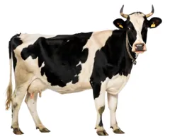
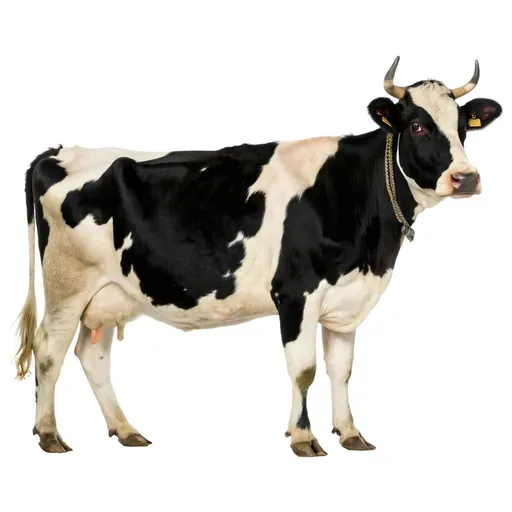
For example, many dairy cows have their horns removed, so for such a cow the fact no longer holds. As the rule no longer applies, the system cannot conclude , although anyone looking at the animal can see that it is still a cow (Figure 3). The rule also fails the other way: a female goat has horns, an udder, hooves and a tail, so the system concludes that it is a cow. Each fix is another rule someone has to think of, and there is always one more exception.
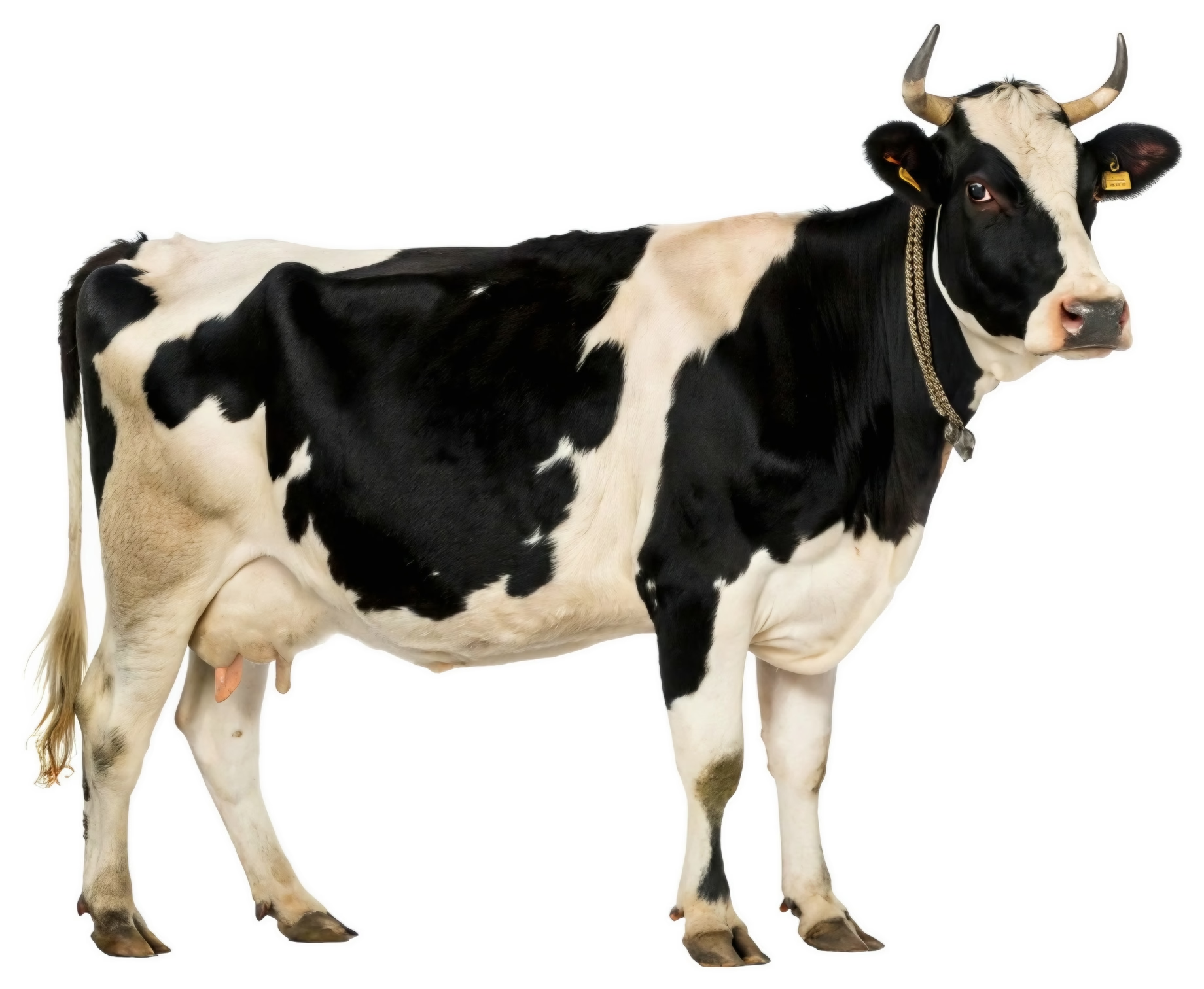
(a) The rule concludes .
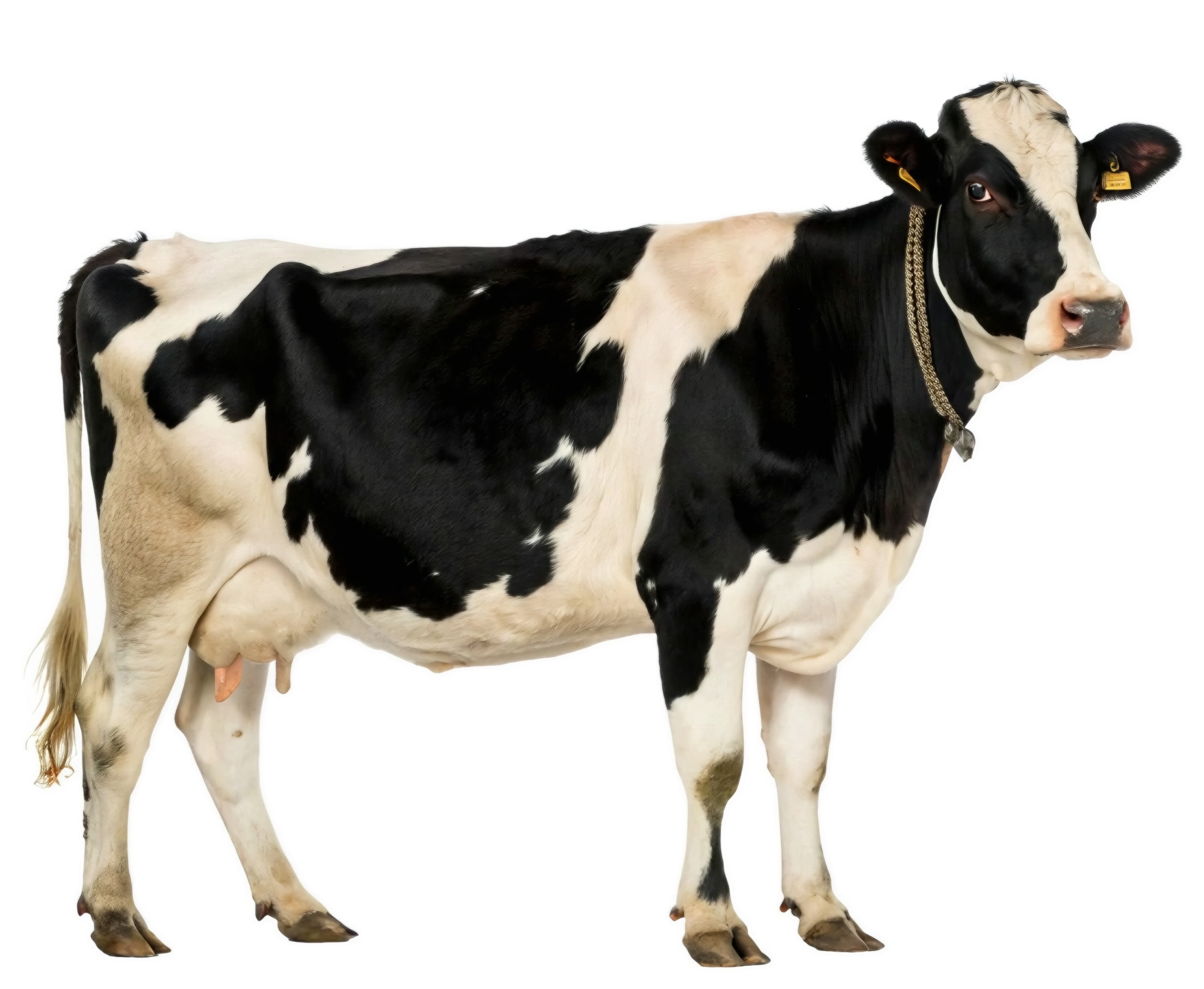
(b) fails, and the rule concludes nothing.
Try fixing the rule yourself (Figure 4).
∀x ( ∧ ∧ ∧ → Cow(x) )
| Animal | Horns | Udder | Hooves | Tail | The rule concludes |
|---|---|---|---|---|---|
| The Holstein | ✓ | ✓ | ✓ | ✓ | Cow(x) ✓ |
| The same cow, dehorned | – | ✓ | ✓ | ✓ | nothing ✗ |
| A female goat | ✓ | ✓ | ✓ | ✓ | Cow(x) ✗ |
| A dog | – | – | – | ✓ | nothing ✓ |
Right about 2 of 4. Click a condition to leave it out of the rule, or to put it back.
Subsymbolic AI
In the end, every AI system works with numbers (and eventually 1s and 0s). In symbolic systems, a person first defines symbols and attaches a meaning to them, such as . Subsymbolic systems skip this intermediate step and work directly on the world as raw numbers (Figure 5), none of which means anything by itself. Whatever such a system comes to know about cows, it learns as patterns across many of these numbers, below the level of symbols, hence the name subsymbolic [7Smolensky, P. (1988). On the proper treatment of connectionism. Behavioral and Brain Sciences, 11(1), 1–23. https://doi.org/10.1017/S0140525X00052432].
picture · pixels
1031009973146121…text · tokens
The cow says mooThe 785cow 19362says 2727moo 45871…sound · samples
−0.360.31−0.560.38−0.600.37…video · frames
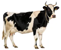
 204 174 146
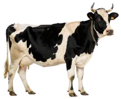
 182
 204
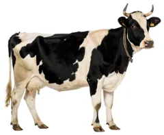 204…
DNA · bases
ATGAAGTGCCTCCTG…A 0T 3G 2A 0A 0G 2…record · fields
- weight
- 650 kg
- milk
- 28 l a day
- age
- 4 years
- horns
- yes
weight 650milk 28age 4horns 1…
Guess first
A random forest sorts e-mails into spam and not spam. It learned from a million e-mails that people had labelled. Is it symbolic or subsymbolic?
How sure are you?
The field comprises a broad spectrum of approaches: classical statistical methods like linear regression [8Maulud, D., & Abdulazeez, A. M. (2020). A Review on Linear Regression Comprehensive in Machine Learning. Journal of Applied Science and Technology Trends, 1(2). https://api.semanticscholar.org/CorpusID:231748167], ensemble techniques such as random forests [9Breiman, L. (2001). Random Forests. Machine Learning, 45(1), 5–32. https://doi.org/10.1023/A:1010933404324] and, arguably, the most prominent paradigm, artificial neural networks.
Unlike in a symbolic system, the knowledge of a subsymbolic system no longer sits in rules anyone can read, but is spread across learned values, the model's parameters. The model learns whatever patterns tell its examples apart, whether or not they are the ones we meant. Additionally, a learned model cannot simply be told what it got wrong.
For example: a neural network trained to recognise cows from photos taken mostly on green pastures may learn that a cow comes with grass around it. Shown a cow standing on a beach, it can fail to recognise the cow [10Beery, S., Van Horn, G., & Perona, P. (2018). Recognition in Terra Incognita. Proceedings of the European Conference on Computer Vision (ECCV).]. There is no rule to correct; the only remedy is to show it more cows in other places, train it again, and check whether it now picks the pattern we meant.
| Symbolic | Subsymbolic | |
|---|---|---|
| Where the knowledge comes from | rules people write | examples |
| Can you read why it decided? | yes | hardly |
| How you correct it | change the rule | train on other examples |
| Cases nobody thought of beforehand | usually fails | often handles them |
As we will see below, generative AI lives entirely on the subsymbolic side. Approaches that bridge the two worlds are commonly referred to as neuro-symbolic or bilateral AI.
Generative vs. Discriminative Models
Machine intelligence is commonly realized through two aims: building discriminative models or generative models (Figure 7) [11Ng, A. Y., & Jordan, M. I. (2001). On discriminative vs. generative classifiers: a comparison of logistic regression and naive Bayes. Proceedings of the 14th International Conference on Neural Information Processing Systems: Natural and Synthetic, NIPS’01, 841–848.].
Guess first
You want a model that tells whether a photo shows a cow. What does it need to learn from?
How sure are you?
Think about how a child learns what a cow is. Someone points. A tree: not a cow. A donkey: not a cow. A black-and-white Holstein: a cow. A goat, with horns: not a cow. The same Holstein without horns: still a cow. With every example the child moves a mental line between what is a cow and what is not. After enough examples the line sits where it should. This decision boundary is what discriminative models learn.
- Class A
- Class B
(a) Linear
- Class A
- Class B
(b) Non-linear
Now put yourself back into art class, where the teacher asks you to draw a cow. You will probably start out poorly, but with every drawing and correction you learn more of what a cow looks like (Figure 9), and that is what a generative model learns.


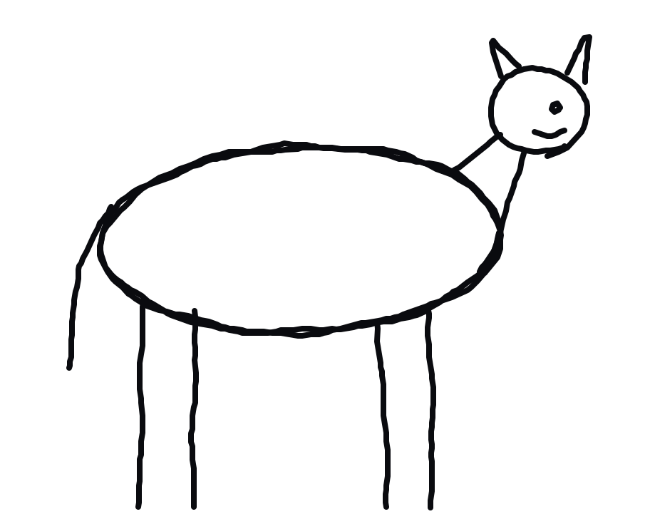
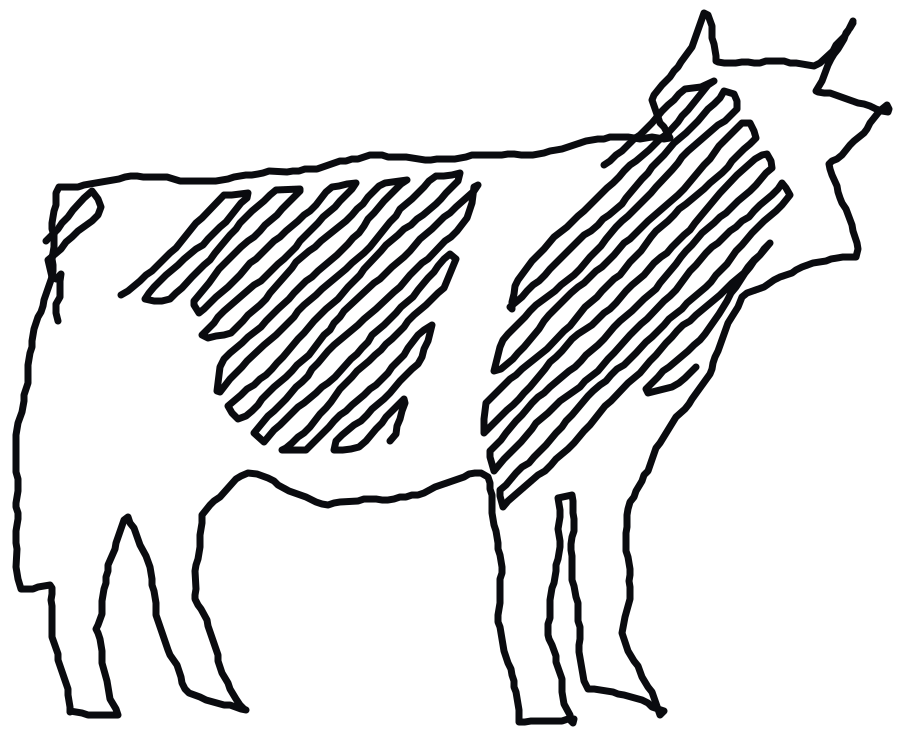
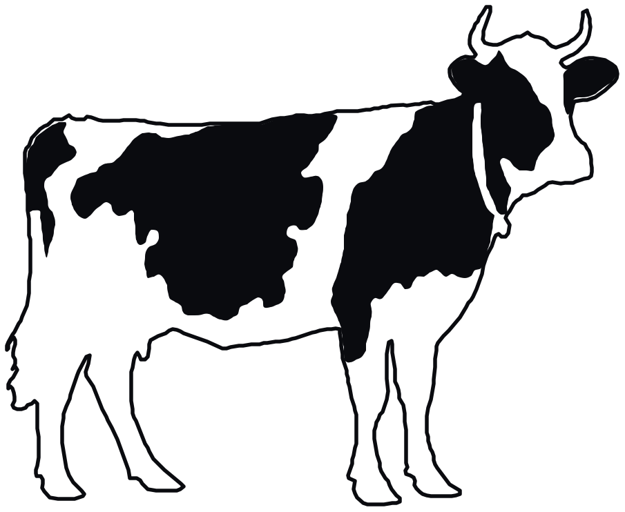
- Puppies
- Kittens
(a) Discriminative Models
- Puppies
- Kittens
- New sample
(b) Generative Models
The probabilistic view
A fundamental stance behind the majority of state-of-the-art machine learning systems is that intelligence can manifest in knowing probability distributions and that regularities of the world show up as differences in probability [12Jaynes, E. T. (2003). Probability Theory: The Logic of Science. Cambridge University Press. https://doi.org/10.1017/CBO9780511790423, 13Shannon, C. E. (1948). A Mathematical Theory of Communication. Bell System Technical Journal, 27(3), 379–423. https://doi.org/10.1002/j.1538-7305.1948.tb01338.x, 14Solomonoff, R. J. (1964). A Formal Theory of Inductive Inference. Part I. Information and Control, 7(1), 1–22. https://doi.org/10.1016/S0019-9958(64)90223-2, 15Sutskever, I., & Patel, D. (2023, March 27). Ilya Sutskever (OpenAI Chief Scientist) – Building AGI, Alignment, Future Models, Spies, Microsoft, Taiwan, & Enlightenment. Dwarkesh Podcast. https://www.dwarkesh.com/p/ilya-sutskever]. For instance, if a small language model, Qwen3-0.6B-Base, finds "The cow says moo" about four times as likely as "The cow says meow", it has some understanding of what cows say.
Joint, conditional and marginal probabilities
Take two random variables, for the animal an audio-sensor records and for the sound the sensor hears at that moment. Their joint distribution — spoken “probability of and ” — gives every pair a probability, such as or , and all of them add up to 1. Everything else follows from it:
- The marginal — spoken “probability of ” — forgets about : how likely each animal is, whatever the sound. It is the sum over every value of , .
- The conditional — spoken “probability of given ” — is the distribution of once is known: what a cow says. It takes the joint probabilities of that and divides them by their sum, so that they add up to 1 again:
Figure 12 has all three for a sensor on a farm.
| animal ↓ · sound → | sum | ||||
|---|---|---|---|---|---|
| 14 % | 1 % | 1 % | 24 % | 40 % | |
| 1 % | 12 % | 1 % | 16 % | 30 % | |
| 1 % | 1 % | 10 % | 18 % | 30 % | |
| sum | 16 % | 14 % | 12 % | 58 % | 100 % |
p(sound | animal = cow)
- moo 35 %
- woof 3 %
- meow 3 %
- nothing 60 %
Read the other way round, this is the product rule, : the probability of both is that of the first, times that of the second given the first. And since the same holds with and swapped, a conditional can be turned around, which is Bayes' rule:
Guess first
The sensor hears a moo. How likely is it that a cow is in front of it?
How sure are you?
A discriminative model learns the conditional probability , where denotes the set of all possible input features2 and is the set of possible labels: how likely “cow” is, given the picture. Its decision boundary (Figure 8) runs where the classes are equally likely.
A generative model, in contrast, learns the distribution of the data itself, : how likely the picture is. Where the data come with labels, the labels are part of it, so that is the joint probability over all possible combinations [11Ng, A. Y., & Jordan, M. I. (2001). On discriminative vs. generative classifiers: a comparison of logistic regression and naive Bayes. Proceedings of the 14th International Conference on Neural Information Processing Systems: Natural and Synthetic, NIPS’01, 841–848.]. It generates new data points by sampling instances from the learned distribution, the likely ones more often than the unlikely.
Autoregression vs. Diffusion
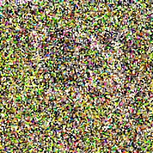
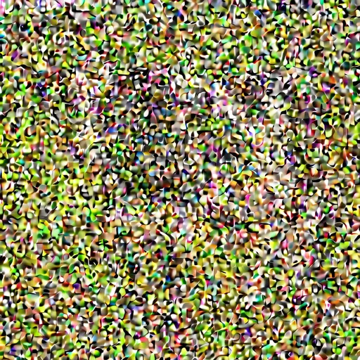
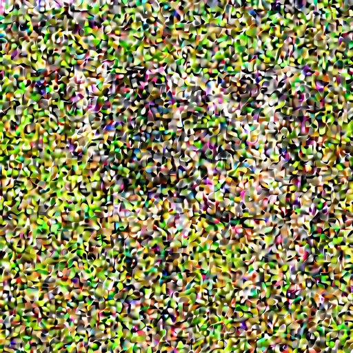
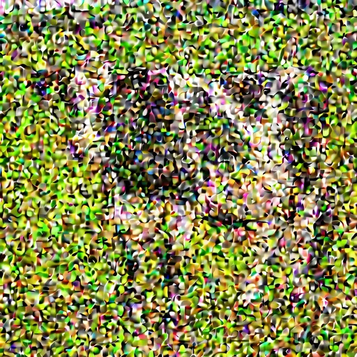
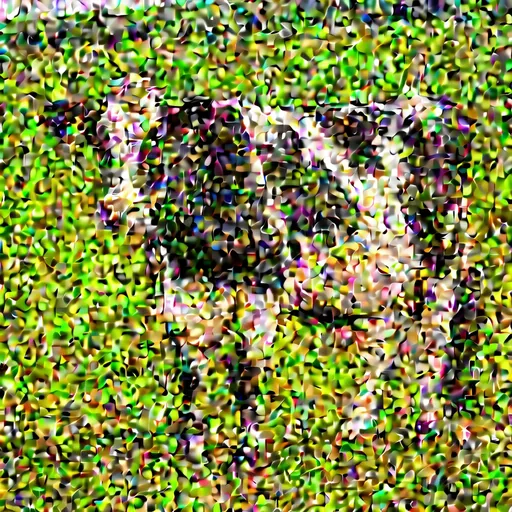
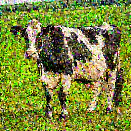
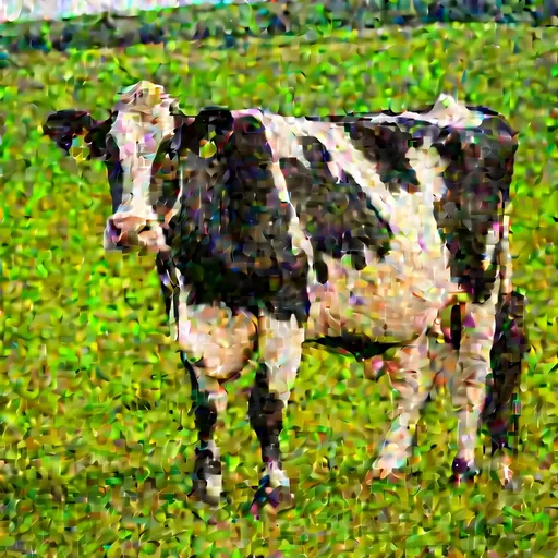
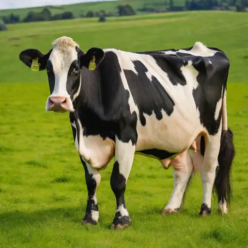
Generative models mainly use one of two techniques to approximate : autoregressive next-token prediction and diffusion (Figure 13).
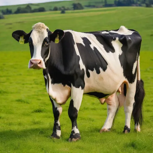
Piece by piece
autoregressive
All at once
diffusion
Autoregression: piece by piece
Almost any data can be read as a sequence: a text as its tokens, a picture as small patches in reading order, a sound as its samples, a video as the patches of one frame after another, a strand of DNA as its bases. Whatever the modality, it becomes . An autoregressive model predicts the next element of such a sequence from all the elements before it:
To generate, it draws from this distribution, appends it to the sequence, and predicts from the longer sequence, which now contains what the model has just made itself. The name says exactly that: auto, from the Greek autós, "self", because it predicts from its own output; regressive, from the Latin regressus, "a going back", because it predicts a value from the values before it, as autoregressive models of a time series do.
- The
- ·cow
- 41 %
- 12 %
- 10 %
- 7.0 %
- 5.0 %
- other 25 %
The product rule, applied again and again, gives the probability of a whole sequence from the probabilities of its parts. The probability of three tokens is that of the first, times that of the second given the first, times that of the third given both:
and in general, for a sequence of tokens, the chain rule:
Every factor is exactly what an autoregressive model predicts: the next token, given all the ones before it. So a model that autoregressively predicts the next token indicrectly models p(x) of the whole sequence.
Tokens, for every modality
An autoregressive model picks its next piece from a fixed list, its vocabulary, so before it can model anything, its data has to become a sequence of tokens. For text that is what a tokenizer does. Pictures and sound are cut into pieces in the same spirit: into patches and into windows.
Text: byte-pair encoding
Most of today's language models learn their vocabulary with byte-pair encoding [16Sennrich, R., Haddow, B., & Birch, A. (2016). Neural Machine Translation of Rare Words with Subword Units. In K. Erk & N. A. Smith (Eds.), Proceedings of the 54th Annual Meeting of the Association for Computational Linguistics (Volume 1: Long Papers) (pp. 1715–1725). Association for Computational Linguistics. https://doi.org/10.18653/v1/P16-1162], in the version that starts from bytes [17Radford, A., Wu, J., Child, R., Luan, D., Amodei, D., & Sutskever, I. (2019). Language Models are Unsupervised Multitask Learners.]. It takes a text, the corpus — normally a huge one. It splits the corpus into words, with the whitespace belonging to the word after it (shown as ·), and every word into its bytes: one for most letters, more for others, like the two of é. Then it counts which two neighbouring units occur together most often and merges them into one new unit, which can itself be merged again later when it happens to be part of a recurring sequence. And repeats (Figure 15).
The vocabulary is the 256 possible bytes, then every merge in the order it was learned, then a few special tokens, for instance one that marks the end of a text. To encode a new text, the tokenizer applies the merges in the same order. Since every text is made of bytes, nothing is ever out of the vocabulary: a character too rare to be merged, such as the 牛 in Figure 15, simply stays three bytes. Qwen3's vocabulary, for one, has 151,669 tokens: the 256 bytes, 151,387 merges and 26 special tokens.
Pictures: patches
To a machine a picture is a grid of pixels, three numbers each: red, green and blue. A vision transformer cuts it into square patches — 16 × 16 pixels in the original [18Dosovitskiy, A., Beyer, L., Kolesnikov, A., Weissenborn, D., Zhai, X., Unterthiner, T., Dehghani, M., Minderer, M., Heigold, G., Gelly, S., Uszkoreit, J., & Houlsby, N. (2021). An Image is Worth 16x16 Words: Transformers for Image Recognition at Scale. International Conference on Learning Representations.] — and reads them row by row, a sequence like a sentence's tokens. Each patch is flattened, its pixels one after the other: 8 × 8 pixels make 8 × 8 × 3 = 192 numbers, . One learned matrix , the same for every patch, turns those numbers into a vector , the patch's embedding. Added to it is where the patch was, , today by row and column, so pictures of any size and shape can be read (Figure 16).
the picture, cut into patches and read row by row
 12345678910111213141516
patch 6 / 16
8 × 8 pixels
xi ∈ ℝ192 its pixels one after another, three numbers each
× W ∈ ℝd×192 one learned matrix, the same for every patch
+ pi = (2, 2) plus where it was: row, column
– optional: the ID of the nearest codebook vector (K = 4,096)
the picture as a sequence, one token a patch
- –
- –
- –
- –
- –
- –
- –
- –
- –
- –
- –
- –
- –
- –
- –
- –
W and the codebook here are random stand-ins, not learned: the steps are real, the numbers only show them.
These are the picture's tokens: vectors, with no IDs and no vocabulary, and for understanding a picture that is enough. To generate a picture token by token, though, the model has to pick its next token from a vocabulary. So each vector is snapped to the nearest of a codebook's vectors, and the picture becomes a sequence of their numbers, IDs like a text's [19van den Oord, A., Vinyals, O., & Kavukcuoglu, K. (2017). Neural Discrete Representation Learning. Advances in Neural Information Processing Systems, 30.]. Emu3's codebook, for instance, has 32,768 entries, and it reads video the same way, a code for 8 × 8 pixels through 4 frames [20Wang, X., & others. (2024). Emu3: Next-Token Prediction is All You Need. arXiv Preprint arXiv:2409.18869.]. An ID's number means nothing in itself: 7554 is not near 7555.
Sound: windows
A sound is a waveform: the air pressure, numbers a second for seconds, — 24,000 a second in the EnCodec codec, 44,100 on a CD. It is cut into windows, the patches of sound: EnCodec's are 320 samples, 13 milliseconds, so 75 a second. A learned encoder turns each window into a vector , and for understanding sound, or for diffusion, the vectors are where it stops. To generate sound token by token, each vector is again snapped to the nearest entry of a codebook, its ID one token a window (Figure 17).
10 samples a window, 16 windows
x ∈ ℝfs·T = ℝ160 the sound, fₛ samples a second for T seconds
Encoder
zt ∈ ℝd one vector a window, 6 of d drawn
optional: the ID of the nearest codebook entry; each further codebook matches what is still missing (K = 1,024)
- 166
- 166
- 799
- 232
- 604
- 681
- 677
- 232
- 681
- 89
- 232
- 374
- 943
- 232
- 826
- 85
window 4 / 16
The encoder and the codebooks here are random stand-ins, not learned: the steps are real, the numbers only show them.
A codebook of 1,024 entries is far too coarse for sound. So codecs repeat it on what is still missing — the vector minus the entry it was snapped to — with a new codebook each time: residual vector quantisation [21Zeghidour, N., Luebs, A., Omran, A., Skoglund, J., & Tagliasacchi, M. (2021). SoundStream: An End-to-End Neural Audio Codec. arXiv Preprint arXiv:2107.03312., 22Défossez, A., Copet, J., Synnaeve, G., & Adi, Y. (2022). High Fidelity Neural Audio Compression. arXiv Preprint arXiv:2210.13438.]. With eight codebooks a window gets 8 IDs; 75 windows a second make 600 IDs, each 10 bits: 6 kilobits a second, where an MP3 takes 128. A single codebook as precise would need entries. The first codebook carries most of what is said; the later ones, how it sounds.
Diffusion: all at once
A diffusion model does not cut its output into pieces. It starts with the whole of it as noise and in every step changes every part at once, so that the whole becomes a little less noisy, until no noise is left.
What noise is depends on the data. For pictures, sound and video it is Gaussian noise added to the signal itself [23Ho, J., Jain, A., & Abbeel, P. (2020). Denoising Diffusion Probabilistic Models. In H. Larochelle, M. Ranzato, R. Hadsell, M. F. Balcan, & H. Lin (Eds.), Advances in Neural Information Processing Systems (Vol. 33, pp. 6840–6851). Curran Associates, Inc. https://proceedings.neurips.cc/paper_files/paper/2020/file/4c5bcfec8584af0d967f1ab10179ca4b-Paper.pdf]; today's models such as Stable Diffusion add it to a compressed version of the signal, a latent, rather than to the pixels. For text it is masks: the noisier a sentence, the more of its tokens are masked. For DNA, each base becomes a probability over A, C, G and T, which is uniform when the base is pure noise. Diffusion, like autoregression, is not tied to one modality.
Learning. The network learns one thing only: to predict the noise in a noisy example. To train it, we take a real cow, draw noise ourselves, and mix the two: a cow plus noise is a noisy cow (Figure 18). How much noise goes in is set by a noise level, from none at all, the cow itself, to so much that nothing but noise is left. This noising is called forward diffusion [24Sohl-Dickstein, J., Weiss, E., Maheswaranathan, N., & Ganguli, S. (2015). Deep Unsupervised Learning using Nonequilibrium Thermodynamics. In F. Bach & D. Blei (Eds.), Proceedings of the 32nd International Conference on Machine Learning (Vol. 37, pp. 2256–2265). PMLR. https://proceedings.mlr.press/v37/sohl-dickstein15.html]. It is fixed: nothing in it is learned. Every training example gets a fresh noise level and fresh noise. Because we drew the noise ourselves, we can compare the network's guess with it, and train the network to make the difference small [23Ho, J., Jain, A., & Abbeel, P. (2020). Denoising Diffusion Probabilistic Models. In H. Larochelle, M. Ranzato, R. Hadsell, M. F. Balcan, & H. Lin (Eds.), Advances in Neural Information Processing Systems (Vol. 33, pp. 6840–6851). Curran Associates, Inc. https://proceedings.neurips.cc/paper_files/paper/2020/file/4c5bcfec8584af0d967f1ab10179ca4b-Paper.pdf].
+ = the data, x₀
× 0.63
noise we drew, ε
× 0.78
the noisy picture, xₜ
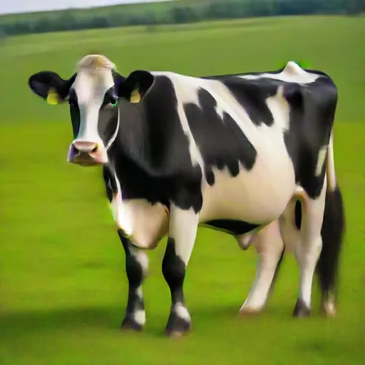
Generating. Backward diffusion starts from pure noise. The network predicts the noise in it; a scaled part of that prediction is subtracted, and the result is a little less noisy. The same network then predicts the noise in the result, and so on, iteratively, until the noise is gone (Figure 19). This loop is run around the network by a sampler; it is not a second thing the network learns.
Why not jump to the end at once? From the noise the network predicts, the clean picture can be worked out in a single step, and samplers do work it out at every step: it is the model's current guess at the finished picture (Figure 19, bottom row). But from a picture that is almost all noise, the best guess is a blur, an average of every cow that could lie under that noise. So each step moves only a little of the way towards the guess, and the next guess, made from a picture with a little less noise, can be a little sharper. The coarse shape is settled first and the details last. The original models took 1,000 such steps [23Ho, J., Jain, A., & Abbeel, P. (2020). Denoising Diffusion Probabilistic Models. In H. Larochelle, M. Ranzato, R. Hadsell, M. F. Balcan, & H. Lin (Eds.), Advances in Neural Information Processing Systems (Vol. 33, pp. 6840–6851). Curran Associates, Inc. https://proceedings.neurips.cc/paper_files/paper/2020/file/4c5bcfec8584af0d967f1ab10179ca4b-Paper.pdf]; today's samplers typically need 20 to 50. Some models predict the clean picture, or a mix of picture and noise, instead of the noise itself; since each of these determines the others, the idea stays the same.
the picture at this step, xₜ
its guess at the finished picture
step 0
step 3
step 6
step 12
step 24
step 50